Advanced Topics

This guide covers advanced statistical concepts, experimental designs, and optimization techniques for sophisticated users of GeoStep.

System Architecture Overview

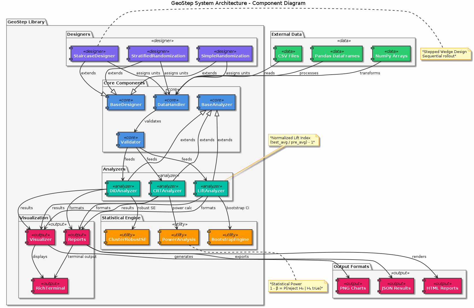Figure: Component architecture of the GeoStep library showing the modular design with analyzers (LiftAnalyzer, DiDAnalyzer, CRTAnalyzer), designers (SimpleRandomization, Stratified, Staircase), and supporting utilities for data handling, visualization, and reporting.

🧮 Statistical Methodology Deep Dive

Randomized Controlled Trials (RCTs) Theory

Fundamental Assumptions

1. SUTVA (Stable Unit Treatment Value Assumption): Treatment of one unit doesn’t affect outcomes of other units

2. Ignorability: Treatment assignment is independent of potential outcomes

3. Positivity: All units have non-zero probability of receiving any treatment

Mathematical Framework

For geographic unit $i$ in time period $t$:

Y_it(1) = potential outcome under treatment
Y_it(0) = potential outcome under control
τ_i = Y_it(1) - Y_it(0) = individual treatment effect
ATE = E[τ_i] = average treatment effect

The randomization ensures:

E[Y_it(1)|T_i = 1] = E[Y_it(1)|T_i = 0]
E[Y_it(0)|T_i = 1] = E[Y_it(0)|T_i = 0]

Normalization Method Details

GeoStep uses a normalized lift index approach:

1. Pre-period normalization:

   baseline_i = mean(Y_it for t in pre_period)
   

2. Expected performance:

   expected_it = baseline_i * seasonal_factor_t
   

3. Lift index calculation:

   lift_index_i = (actual_i - expected_i) / expected_i
   

4. Treatment effect estimation:

   ATE = mean(lift_index_treatment) - mean(lift_index_control)
   

This approach is robust to:

• Scale differences between geographic units

• Seasonal patterns in the data

• Natural growth trends

Power Analysis Mathematics

Statistical power is the probability of detecting a true effect:

Power = P(reject H0 | H1 is true)
     = P(|t-statistic| > critical_value | true_effect ≠ 0)

For a two-sample t-test with effect size δ:

Power = Φ(δ√(n/2) - z_α/2) + Φ(-δ√(n/2) - z_α/2)

Where:

• Φ = standard normal CDF

• δ = standardized effect size

• n = sample size per group

• z_α/2 = critical value for significance level α

🏗️ Advanced Experimental Designs

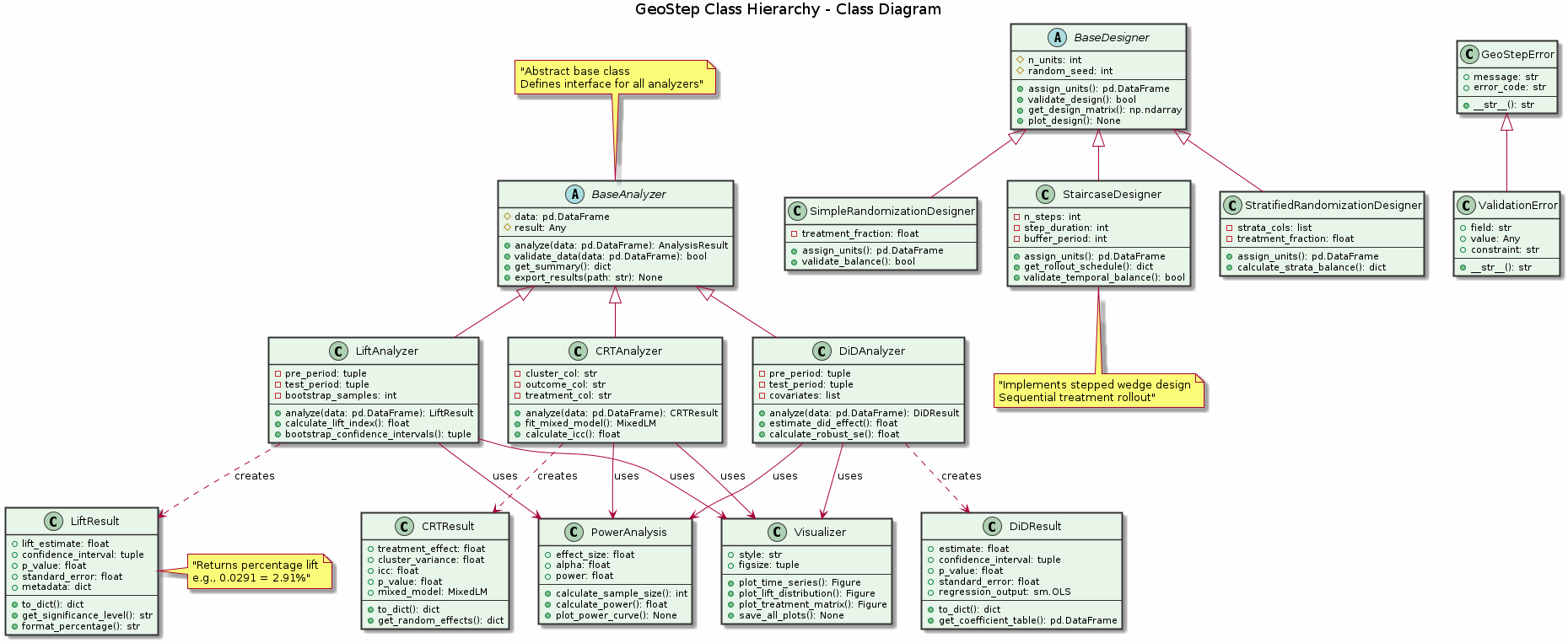Figure: Object-oriented class hierarchy showing inheritance relationships. BaseAnalyzer and BaseDesigner serve as abstract base classes, with concrete implementations for different analysis methods and experimental designs.

Stepped-Wedge Trials

Design Matrix

For a stepped-wedge with K clusters and T time periods:

import numpy as np

def create_stepped_wedge_matrix(K, T, step_size=1):
    """
    Creates a stepped-wedge design matrix.
    
    Parameters:
    K: Number of clusters
    T: Number of time periods
    step_size: Number of clusters switching per step
    """
    design = np.zeros((K, T))
    
    # Calculate switch times
    switch_times = np.arange(1, T, T//K)
    
    for i, switch_time in enumerate(switch_times):
        cluster_start = i * step_size
        cluster_end = min((i + 1) * step_size, K)
        design[cluster_start:cluster_end, switch_time:] = 1
    
    return design

Analysis Model

Mixed-effects model for stepped-wedge:

Y_ijt = β0 + β1*X_jt + α_j + γ_t + ε_ijt

Where:

• Y_ijt = outcome for individual i in cluster j at time t

• X_jt = treatment indicator (0/1)

• α_j = cluster random effect

• γ_t = time fixed effect

• β1 = treatment effect (parameter of interest)

Staircase Design Optimization

Optimal Allocation

For a staircase design, the optimal number of pre/post periods balances:

• Statistical power (more periods = better)

• Operational cost (fewer periods = cheaper)

def optimize_staircase_design(total_budget, cost_per_period, 
                             effect_size, alpha=0.05, power=0.8):
    """
    Find optimal pre/post period allocation for staircase design.
    """
    best_power = 0
    best_design = None
    
    for pre_periods in range(2, 10):
        for post_periods in range(2, 10):
            total_cost = (pre_periods + post_periods) * cost_per_period
            
            if total_cost <= total_budget:
                # Calculate power for this design
                power = calculate_staircase_power(
                    pre_periods, post_periods, effect_size, alpha
                )
                
                if power > best_power:
                    best_power = power
                    best_design = (pre_periods, post_periods)
    
    return best_design, best_power

Cluster Randomized Trials (CRTs)

Intracluster Correlation (ICC)

The ICC measures similarity within clusters:

ICC = σ²_between / (σ²_between + σ²_within)

Higher ICC reduces effective sample size:

Design_Effect = 1 + (m - 1) * ICC
Effective_n = n / Design_Effect

Where m = average cluster size.

Sample Size Calculation

For CRTs, required number of clusters:

def calculate_crt_sample_size(effect_size, icc, cluster_size, 
                             alpha=0.05, power=0.8):
    """
    Calculate required number of clusters for CRT.
    """
    from scipy import stats
    
    z_alpha = stats.norm.ppf(1 - alpha/2)
    z_beta = stats.norm.ppf(power)
    
    design_effect = 1 + (cluster_size - 1) * icc
    
    n_clusters = (2 * design_effect * (z_alpha + z_beta)**2) / \
                 (cluster_size * effect_size**2)
    
    return int(np.ceil(n_clusters))

⚡ Performance Optimization

Large-Scale Experiments

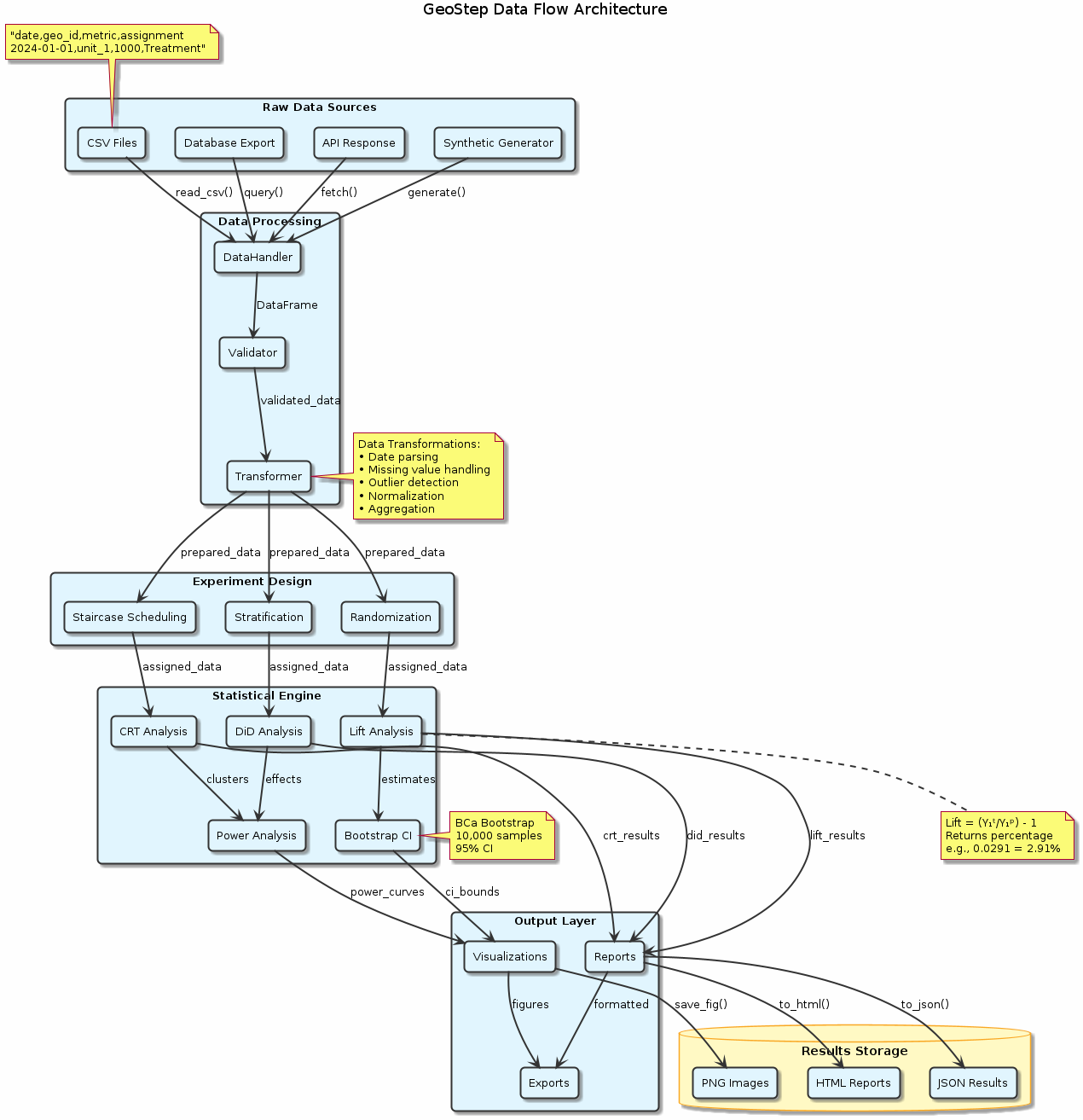Figure: End-to-end data flow from raw sources through processing pipeline to final outputs. The architecture supports multiple data formats and provides both programmatic and visual outputs for comprehensive analysis.

Data Sampling for Power Analysis

For datasets with millions of rows:

def stratified_sample_for_power(df, geo_col, strata_col, 
                               sample_size=50000):
    """
    Create stratified sample for power analysis.
    """
    # Calculate strata proportions
    strata_props = df[strata_col].value_counts(normalize=True)
    
    sampled_data = []
    for stratum, prop in strata_props.items():
        stratum_data = df[df[strata_col] == stratum]
        stratum_sample_size = int(sample_size * prop)
        
        if len(stratum_data) > stratum_sample_size:
            stratum_sample = stratum_data.sample(
                n=stratum_sample_size, 
                random_state=42
            )
        else:
            stratum_sample = stratum_data
            
        sampled_data.append(stratum_sample)
    
    return pd.concat(sampled_data, ignore_index=True)

Parallel Processing Configuration

import os
from joblib import Parallel, delayed

# Configure parallel processing
os.environ['NUMBA_NUM_THREADS'] = '8'  # Limit CPU usage
os.environ['OMP_NUM_THREADS'] = '8'

# Custom parallel power analysis
def parallel_power_analysis(historical_data, effect_sizes, 
                           test_weeks_list, n_jobs=4):
    """
    Run power analysis with custom parallelization.
    """
    def single_scenario(effect, weeks):
        return run_single_power_scenario(
            historical_data, effect, weeks
        )
    
    scenarios = [(e, w) for e in effect_sizes 
                 for w in test_weeks_list]
    
    results = Parallel(n_jobs=n_jobs)(
        delayed(single_scenario)(effect, weeks) 
        for effect, weeks in scenarios
    )
    
    return pd.DataFrame(results)

Memory Optimization

Efficient Data Types

def optimize_datatypes(df):
    """
    Optimize DataFrame memory usage.
    """
    # Convert object columns to category
    for col in df.select_dtypes(include=['object']):
        if df[col].nunique() < 0.5 * len(df):
            df[col] = df[col].astype('category')
    
    # Downcast numeric types
    for col in df.select_dtypes(include=['int64']):
        df[col] = pd.to_numeric(df[col], downcast='integer')
    
    for col in df.select_dtypes(include=['float64']):
        df[col] = pd.to_numeric(df[col], downcast='float')
    
    return df

🔬 Advanced Analysis Techniques

Sensitivity Analysis

Robustness Checks

def sensitivity_analysis(df, geo_col, assignment_col, 
                        date_col, kpi_col, test_start):
    """
    Perform sensitivity analysis.
    """
    results = {}
    
    # 1. Different pre-period lengths
    for pre_weeks in [4, 6, 8, 10, 12]:
        pre_end = pd.to_datetime(test_start) - pd.Timedelta(days=1)
        pre_start = pre_end - pd.Timedelta(weeks=pre_weeks)
        
        subset_data = df[df[date_col] >= pre_start]
        result = run_primary_analysis(subset_data, ...)
        results[f'pre_weeks_{pre_weeks}'] = result
    
    # 2. Outlier removal
    for percentile in [95, 97.5, 99]:
        threshold = df[kpi_col].quantile(percentile/100)
        clean_data = df[df[kpi_col] <= threshold]
        result = run_primary_analysis(clean_data, ...)
        results[f'outlier_removal_{percentile}'] = result
    
    # 3. Different analysis methods
    results['primary'] = run_primary_analysis(df, ...)
    results['did'] = run_did_analysis(df, ...)
    
    return results

Bayesian Analysis

Bayesian Treatment Effect Estimation

import pymc as pm
import arviz as az

def bayesian_rct_analysis(treatment_data, control_data):
    """
    Bayesian analysis of RCT results.
    """
    with pm.Model() as model:
        # Priors
        mu_control = pm.Normal('mu_control', mu=0, sigma=1)
        mu_treatment = pm.Normal('mu_treatment', mu=0, sigma=1)
        sigma = pm.HalfNormal('sigma', sigma=1)
        
        # Likelihood
        control_obs = pm.Normal('control_obs', 
                               mu=mu_control, 
                               sigma=sigma, 
                               observed=control_data)
        
        treatment_obs = pm.Normal('treatment_obs', 
                                 mu=mu_treatment, 
                                 sigma=sigma, 
                                 observed=treatment_data)
        
        # Treatment effect
        treatment_effect = pm.Deterministic(
            'treatment_effect', 
            mu_treatment - mu_control
        )
        
        # Sampling
        trace = pm.sample(2000, tune=1000, 
                         return_inferencedata=True)
    
    return trace

Causal Inference Extensions

Instrumental Variables

For cases with non-compliance:

def instrumental_variables_analysis(df, instrument_col, 
                                   treatment_col, outcome_col):
    """
    Two-stage least squares for IV analysis.
    """
    from sklearn.linear_model import LinearRegression
    
    # First stage: instrument -> treatment
    X_first = df[[instrument_col]]
    y_first = df[treatment_col]
    first_stage = LinearRegression().fit(X_first, y_first)
    
    # Predicted treatment
    treatment_hat = first_stage.predict(X_first)
    
    # Second stage: predicted treatment -> outcome
    X_second = treatment_hat.reshape(-1, 1)
    y_second = df[outcome_col]
    second_stage = LinearRegression().fit(X_second, y_second)
    
    # IV estimate
    iv_estimate = second_stage.coef_[0]
    
    return {
        'iv_estimate': iv_estimate,
        'first_stage_r2': first_stage.score(X_first, y_first),
        'weak_instrument_test': first_stage_r2 > 0.1
    }

🚀 Production Deployment

Automated Experiment Pipeline

Configuration Management

from dataclasses import dataclass
from typing import List, Optional
import yaml

@dataclass
class ExperimentConfig:
    """Configuration for automated experiments."""
    name: str
    geo_col: str
    date_col: str
    kpi_col: str
    treatment_description: str
    expected_effect_size: float
    test_duration_weeks: int
    randomization_method: str = 'simple'
    stratification_vars: Optional[List[str]] = None
    power_threshold: float = 0.8
    
    @classmethod
    def from_yaml(cls, yaml_path: str):
        with open(yaml_path, 'r') as f:
            config_dict = yaml.safe_load(f)
        return cls(**config_dict)

Experiment Orchestration

class ExperimentOrchestrator:
    """Orchestrates end-to-end experiment workflow."""
    
    def __init__(self, config: ExperimentConfig):
        self.config = config
        self.results = {}
    
    def run_full_pipeline(self, data_path: str):
        """Run complete experiment pipeline."""
        
        # 1. Load and validate data
        data = self.load_and_validate_data(data_path)
        
        # 2. Power analysis
        power_results = self.run_power_analysis(data)
        
        # 3. Check if experiment is viable
        if not self.is_experiment_viable(power_results):
            raise ValueError("Experiment not viable - insufficient power")
        
        # 4. Randomization
        assigned_data = self.randomize_units(data)
        
        # 5. Balance check
        balance_results = self.check_balance(assigned_data)
        
        # 6. Generate experiment plan
        self.generate_experiment_plan(assigned_data)
        
        return {
            'power_analysis': power_results,
            'balance_check': balance_results,
            'assignment': assigned_data,
            'experiment_ready': True
        }

Monitoring and Alerting

Real-time Monitoring

def monitor_experiment_execution(experiment_id: str, 
                                data_source: str):
    """
    Monitor experiment execution in real-time.
    """
    import time
    from datetime import datetime, timedelta
    
    while True:
        # Check data freshness
        latest_data = get_latest_data(data_source)
        data_lag = datetime.now() - latest_data['date'].max()
        
        if data_lag > timedelta(days=2):
            send_alert(f"Data lag detected: {data_lag}")
        
        # Check treatment delivery
        treatment_delivery = check_treatment_delivery(
            experiment_id, latest_data
        )
        
        if treatment_delivery['coverage'] < 0.95:
            send_alert(f"Low treatment coverage: {treatment_delivery}")
        
        # Check for contamination
        contamination = check_contamination(latest_data)
        
        if contamination['spillover_detected']:
            send_alert(f"Contamination detected: {contamination}")
        
        time.sleep(3600)  # Check hourly

📊 Advanced Reporting

Interactive Dashboards

import plotly.graph_objects as go
from plotly.subplots import make_subplots

def create_interactive_dashboard(experiment_results):
    """
    Create interactive dashboard for experiment results.
    """
    fig = make_subplots(
        rows=2, cols=2,
        subplot_titles=('Power Analysis', 'Time Series', 
                       'Lift Distribution', 'Balance Check'),
        specs=[[{"type": "heatmap"}, {"type": "scatter"}],
               [{"type": "histogram"}, {"type": "bar"}]]
    )
    
    # Power analysis heatmap
    fig.add_trace(
        go.Heatmap(
            z=experiment_results['power_matrix'],
            colorscale='Viridis'
        ),
        row=1, col=1
    )
    
    # Time series
    fig.add_trace(
        go.Scatter(
            x=experiment_results['dates'],
            y=experiment_results['treatment_trend'],
            name='Treatment'
        ),
        row=1, col=2
    )
    
    # Add more plots...
    
    fig.update_layout(
        title="Experiment Results Dashboard",
        height=800
    )
    
    return fig

This advanced topics guide provides the mathematical foundation and sophisticated techniques needed for complex experimental designs and large-scale implementations of GeoStep.