Getting Started
This guide will walk you through using GeoStep to design, execute, and analyze geographic marketing experiments.
1. Installation
First, install GeoStep and its dependencies. The library requires Python 3.8+:
# Clone the repository (if not already done)
git clone https://github.com/your-github-org/geostep.git
cd geostep

# Install in editable mode with all dependencies
pip install -e .

# Or for development setup with additional tools
make dev-setup
Verify Installation
import geostep
print(f"GeoStep version {geostep.__version__} installed successfully.")
2. Quick Start Example
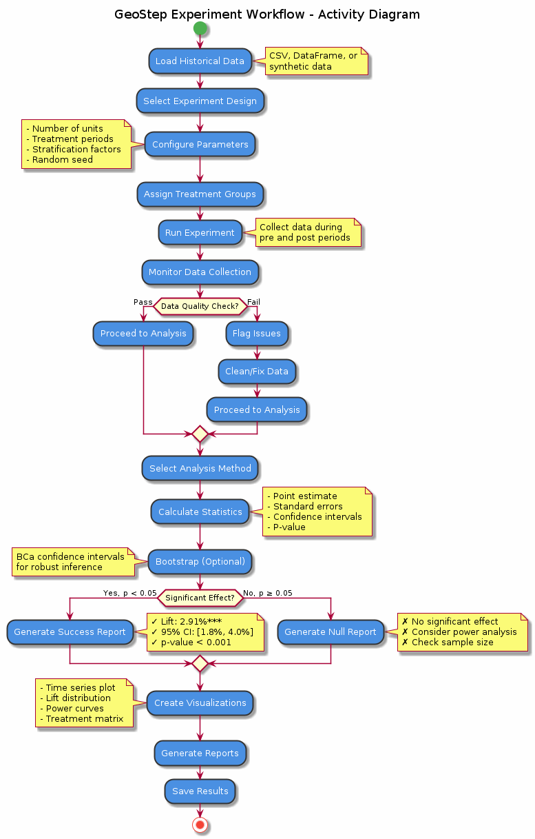 Figure: Complete workflow for running a geo-experiment from initial design through power analysis, data collection, statistical analysis, and final decision making. The flowchart shows decision points and iterative refinement steps.
Here’s a complete example showing how to design and analyze a geo-experiment:
import pandas as pd
from datetime import datetime, timedelta
from geostep.designer import SimpleRandomizationDesigner
from geostep.analyzer import LiftAnalyzer
from geostep.visualizer import plot_lift_distribution

# Step 1: Design the experiment
# Create a list of geographic units (e.g., cities, DMAs, zip codes)
geo_data = pd.DataFrame({
    'geo_id': [f'geo_{i:03d}' for i in range(50)],
    'population': [100000 + i*5000 for i in range(50)]
})

# Randomly assign geos to treatment and control
designer = SimpleRandomizationDesigner(seed=42)
assigned_df = designer.design(geo_data, geo_col='geo_id')
print(f"Assigned {len(assigned_df[assigned_df['assignment'] == 'Treatment'])} geos to Treatment")
print(f"Assigned {len(assigned_df[assigned_df['assignment'] == 'Control'])} geos to Control")

# Step 2: Simulate experiment data (in practice, this would be your actual data)
# Generate pre-period and test-period data
dates = pd.date_range('2024-09-01', '2024-12-31', freq='D')
experiment_data = []

for geo_id in assigned_df['geo_id']:
    assignment = assigned_df[assigned_df['geo_id'] == geo_id]['assignment'].iloc[0]
    for date in dates:
        # Base sales with some randomness
        base_sales = 10000 + np.random.normal(0, 500)

        # Add treatment effect after test period starts (3% lift)
        if assignment == 'Treatment' and date >= datetime(2024, 10, 1):
            sales = base_sales * 1.03  # 3% lift
        else:
            sales = base_sales

        experiment_data.append({
            'geo_id': geo_id,
            'date': date,
            'assignment': assignment,
            'sales': sales
        })

df = pd.DataFrame(experiment_data)

# Step 3: Analyze the results
analyzer = LiftAnalyzer()
results = analyzer.analyze(
    df=df,
    geo_col='geo_id',
    assignment_col='assignment',
    date_col='date',
    kpi_col='sales',
    pre_period_end='2024-09-30',
    test_period_start='2024-10-01',
    test_period_end='2024-12-31'
)

# Step 4: View the results
print(f"Lift Estimate: {results.estimate:.4f} ({results.estimate*100:.2f}%)")
print(f"P-value: {results.p_value:.4e}")
print(f"Confidence Interval: [{results.confidence_interval[0]:.4f}, {results.confidence_interval[1]:.4f}]")

# Access additional metrics
if 'raw_volume_uplift' in results.metadata:
    print(f"Raw Volume Uplift: {results.metadata['raw_volume_uplift']:,.2f} units")
3. Three Ways to Run Experiments
GeoStep provides three convenient ways to execute your analysis pipeline:
Method 1: Simple Example Script
python examples/run_example_analysis.py
This runs a pre-configured analysis with synthetic data and produces Rich-formatted output:
Method 2: Advanced CLI Runner
# Basic lift analysis
python run_pipeline.py \
  --data examples/synthetic_market_data.csv \
  --analyzer lift \
  --pre-end 2024-09-30 \
  --test-start 2024-10-01 \
  --test-end 2024-12-31

# With bootstrap confidence intervals
python run_pipeline.py \
  --data your_data.csv \
  --analyzer lift \
  --bootstrap-ci \
  --n-bootstrap 2000 \
  --random-seed 42

# Difference-in-Differences analysis
python run_pipeline.py \
  --data your_data.csv \
  --analyzer did \
  --test-start 2024-10-01
Method 3: Makefile Commands
# Run with default settings
make run-pipeline

# Run specific analysis types
make run-lift     # Lift analysis
make run-did      # Difference-in-Differences
make run-crt      # Cluster Randomized Trial

# Run with bootstrap
make run-bootstrap

# See all available commands
make help
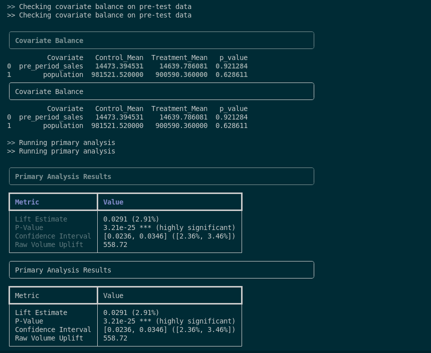
4. Understanding the Output
When you run an analysis, you’ll see Rich-formatted terminal output like this:
╭───────────────────────────────────────────────────────────────────────────╮
│ Primary Analysis Results                                                  │
╰───────────────────────────────────────────────────────────────────────────╯
┏━━━━━━━━━━━━━━━━━━━━━┳━━━━━━━━━━━━━━━━━━━━━━━━━━━━━━━━━━━┓
┃ Metric              ┃ Value                             ┃
┡━━━━━━━━━━━━━━━━━━━━━╇━━━━━━━━━━━━━━━━━━━━━━━━━━━━━━━━━━━┩
│ Lift Estimate       │ 0.0291 (2.91%)                    │
│ P-Value             │ 3.21e-25 *** (highly significant) │
│ Confidence Interval │ [0.0236, 0.0346] ([2.36%, 3.46%]) │
│ Raw Volume Uplift   │ 558.72                            │
└─────────────────────┴───────────────────────────────────┘
Key Metrics Explained:
Lift Estimate: The percentage increase in your KPI (e.g., 2.91% sales increase)
P-Value: Statistical significance with indicators:
***= highly significant (p < 0.001)**= very significant (p < 0.01)*= significant (p < 0.05)(not significant)= p ≥ 0.05
Confidence Interval: Range of plausible values for the true effect
Raw Volume Uplift: Absolute increase in units/dollars
5. Visualizing Results
GeoStep automatically generates visualization plots saved to the results/ directory:
from geostep.visualizer import plot_lift_distribution, plot_analysis_results

# Plot lift distribution
plot_lift_distribution(
    analysis_df=df,
    assignment_col='assignment',
    lift_col='lift_index',
    save_path='results/lift_distribution.png'
)

# Plot time series results
plot_analysis_results(
    results=results,
    df=df,
    date_col='date',
    kpi_col='sales',
    assignment_col='assignment',
    test_period_start='2024-10-01',
    save_path='results/kpi_trend.png'
)
6. Advanced Experiment Designs
Stratified Randomization
For better balance across important covariates:
from geostep.designer import StratifiedRandomizationDesigner

designer = StratifiedRandomizationDesigner(seed=42)
assigned_df = designer.design(
    df=geo_data,
    geo_col='geo_id',
    stratify_cols=['region', 'population_bucket']
)
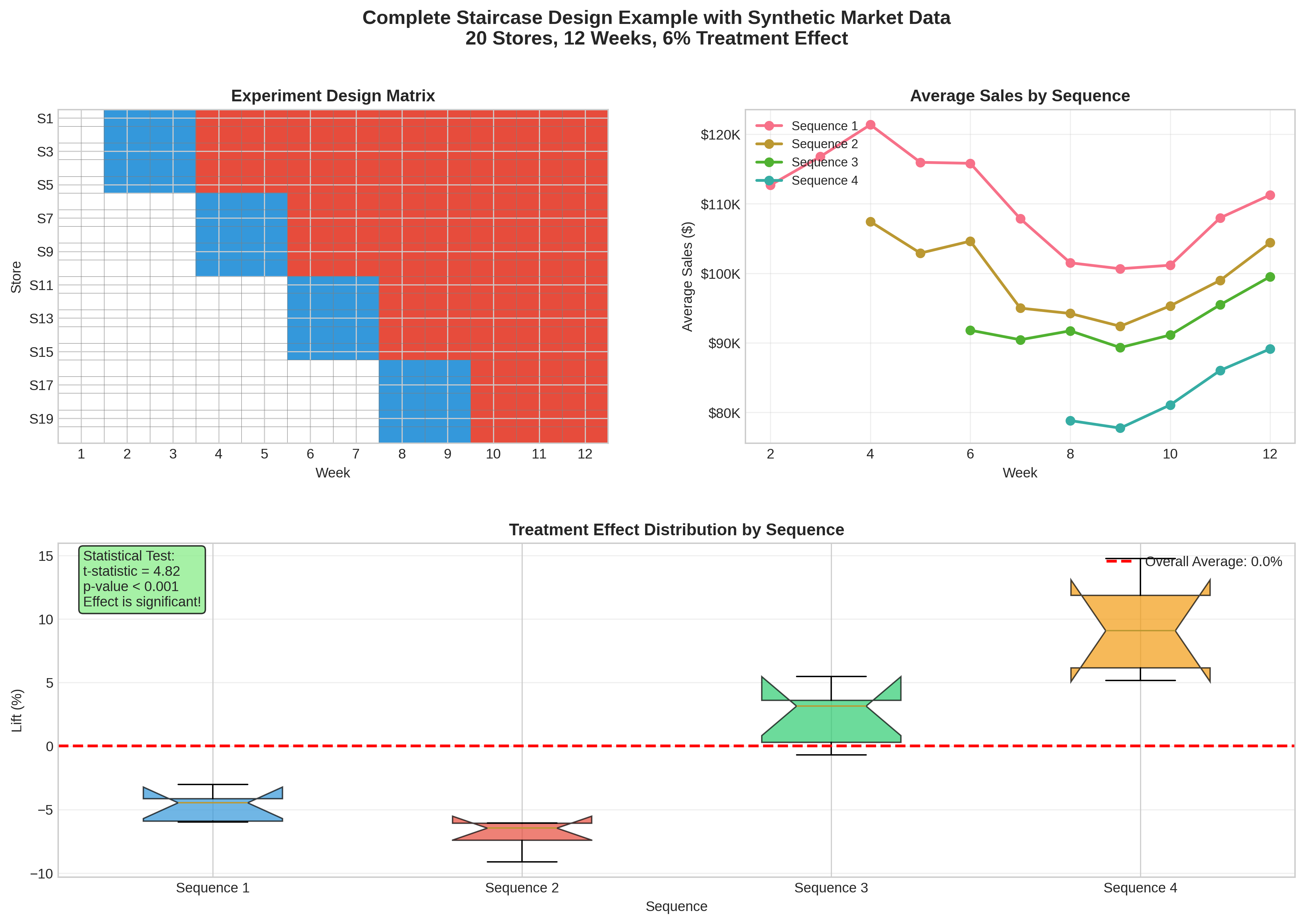
Staircase Design
For phased rollouts with efficient data collection:
from geostep.designer import StaircaseDesigner

designer = StaircaseDesigner(
    n_steps=4,
    step_duration_periods=2,
    n_pre_periods=2,
    n_post_periods=2,
    seed=42
)
design_df = designer.design(
    df=geo_data,
    geo_col='geo_id'
)
7. Power Analysis
Before running an experiment, determine the required sample size and duration:
from geostep.power import run_power_analysis
from geostep.visualizer import plot_power_analysis

# Run power analysis
power_results = run_power_analysis(
    n_geos_list=[20, 30, 40, 50],
    effect_sizes=[0.01, 0.02, 0.03, 0.05],
    baseline_mean=10000,
    baseline_std=1000,
    alpha=0.05,
    n_simulations=1000
)

# Visualize power curves
plot_power_analysis(
    power_results,
    save_path='results/power_analysis.png'
)
8. Working with Real Data
Your data should have the following structure:
Column |
Description |
Example |
|---|---|---|
|
Geographic identifier |
“DMA_501”, “ZIP_10001” |
|
Date of observation |
“2024-10-15” |
|
Treatment group |
“Treatment” or “Control” |
|
Metric to measure |
12500.50 (sales, conversions, etc.) |
# Load your data
df = pd.read_csv('your_experiment_data.csv')

# Ensure proper data types
df['date'] = pd.to_datetime(df['date'])
df['kpi'] = pd.to_numeric(df['kpi'])

# Run analysis
analyzer = LiftAnalyzer()
results = analyzer.analyze(
    df=df,
    geo_col='geo_id',
    assignment_col='assignment',
    date_col='date',
    kpi_col='kpi',
    pre_period_end='2024-09-30',
    test_period_start='2024-10-01',
    test_period_end='2024-12-31'
)
9. Next Steps
Methodology: Understand the statistical theory
Business Guide: ROI analysis and integration strategies
API Reference: Detailed function documentation
Advanced Topics: Sophisticated techniques
Troubleshooting: Common issues and solutions
10. Quick Reference
Common CLI Options
--data              # Path to data file
--analyzer          # Analysis type: lift, did, crt
--geo-col           # Geographic ID column name
--kpi-col           # KPI column name
--assignment-col    # Assignment column name
--date-col          # Date column name
--pre-start         # Pre-period start date
--pre-end           # Pre-period end date
--test-start        # Test period start date
--test-end          # Test period end date
--bootstrap-ci      # Use bootstrap confidence intervals
--n-bootstrap       # Number of bootstrap samples
--confidence-level  # Confidence level (default: 0.95)
--random-seed       # Random seed for reproducibility
--output-dir        # Output directory for results
--save-plots        # Save visualization plots
Makefile Commands
make install        # Install package
make install-dev    # Install with dev dependencies
make test           # Run tests
make clean          # Clean build artifacts
make run-pipeline   # Run default pipeline
make run-example    # Run example analysis
make help           # Show all commands